Roundup of growth chart packages
At rOpenSci’s annual unconf, I suggested a project to work on functions that convert physical growth measurements into z-scores and percentiles. For example, researchers in the United States studying childhood obesity often calculate the BMI z-score or percentage of the 95th percentile of BMI from nationally representative survey data.
During the process of brainstorming and working on this project, the team1 I was working with found out some related R packages that do this. To help us move forward with the project and identify next steps, I round up these packages below.2 If I’m missing something, please comment so I can add it to this post!
Below is an overview of 4 packages: AGD, growthstandards/hgbd, zscorer, and childsds.
Anthropometric data
The National Health and Nutrition Examination Survey (NHANES) has data on height, weight, blood pressure, and other measurements for adolescents from 0 to 239 months that I will use to explore these packages. I’m converting the original variables names to names that are easier to use. The data is in an .xpt file, which I’ll read in using the haven package.
library(tidyverse)## ── Attaching packages ─────────────────────────────────────── tidyverse 1.3.0 ──## ✓ ggplot2 3.3.2 ✓ purrr 0.3.4
## ✓ tibble 3.0.4 ✓ dplyr 1.0.2
## ✓ tidyr 1.1.2 ✓ stringr 1.4.0
## ✓ readr 1.4.0 ✓ forcats 0.5.0## ── Conflicts ────────────────────────────────────────── tidyverse_conflicts() ──
## x dplyr::filter() masks stats::filter()
## x dplyr::lag() masks stats::lag()library(haven)
demo_data <- read_xpt(url("https://wwwn.cdc.gov/Nchs/Nhanes/2015-2016/DEMO_I.XPT"))
demo_need <- demo_data %>%
select(id = SEQN,
agemos = RIDEXAGM,
sex_num = RIAGENDR)
exam_data <- read_xpt(url("https://wwwn.cdc.gov/Nchs/Nhanes/2015-2016/BMX_I.XPT"))
exam_need <- exam_data %>%
select(id = SEQN,
bmi = BMXBMI,
height_cm = BMXHT,
length_cm = BMXRECUM,
weight_kg = BMXWT)
df <- demo_need %>%
left_join(exam_need, by = "id") %>%
filter(!is.na(agemos)) %>%
mutate(sex_mf = if_else(sex_num == 1, "M", "F"),
sex = if_else(sex_num == 1, "Male", "Female"),
# recumbent length is used if under 2 years old
height_length_cm = if_else(agemos < 24, length_cm, height_cm),
ageyears = agemos/12)
# xpt file had column labels, remove column labels
child_df <- df[1:nrow(df), ]AGD
The Analysis of Growth Data (AGD) package is developed by Stef van Buuren. More info here.
Tools for the analysis of growth data: to extract an LMS table from a gamlss object, to calculate the standard deviation scores and its inverse, and to superpose two wormplots from different models. The package contains a some varieties of reference tables, especially for The Netherlands.
It has functions for reference tables from the CDC 2000 growth charts, Third Dutch Growth Study (1980), Fourth Dutch Growth Study (1997), and WHO growth charts. The function y2z() converts measurements into standard deviation scores (z-scores) and z2y() does the opposite, convert standard deviation scores into measurements.
The package is available on CRAN.
install.packages("AGD")To calculate the age- and sex-adjusted BMI z-scores for the children in the NHANES dataset, we can do the following:
library(AGD)

bmi_levels <- c("Underweight", "Healthy weight", "Overweight",
                "Obesity", "Severe obesity")

agd_df <- child_df %>%
  # the CDC growth charts are typically used for children 2 years or older
  filter(agemos >= 24) %>%
  mutate(bmiz =  AGD::y2z(y = bmi, x = ageyears, sex = sex_mf, ref = cdc.bmi),
         bmipct = pnorm(bmiz),
         # what is the 95th percentile for the child's age and sex?,
         z = qnorm(.95),
         p95 = AGD::z2y(z = z, x= ageyears, sex = sex_mf, ref = cdc.bmi),
         # percentage of the 95th percentile
         bmipct95 = bmi/p95,
         # bmi category
         bmicat = factor(case_when(bmipct < .05 ~ "Underweight",
                                   bmipct < .85 ~ "Healthy weight",
                                   bmipct < .95 ~ "Overweight",
                                   bmipct95 < 1.2 ~ "Obesity",
                                   bmipct95 >= 1.2 ~ "Severe obesity"),
                         levels = bmi_levels))

agd_df %>%
  select(agemos, bmi, bmiz, bmipct, bmipct95) %>%
skimr::skim()| Name | Piped data |
| Number of rows | 3426 |
| Number of columns | 5 |
| _______________________ | |
| Column type frequency: | |
| numeric | 5 |
| ________________________ | |
| Group variables | None |
Variable type: numeric
| skim_variable | n_missing | complete_rate | mean | sd | p0 | p25 | p50 | p75 | p100 | hist |
|---|---|---|---|---|---|---|---|---|---|---|
| agemos | 0 | 1.00 | 121.86 | 60.89 | 24.00 | 70.00 | 118.00 | 173.00 | 239.00 | ▇▇▇▆▅ |
| bmi | 86 | 0.97 | 20.32 | 5.71 | 11.50 | 16.20 | 18.60 | 22.80 | 54.70 | ▇▅▁▁▁ |
| bmiz | 3426 | 0.00 | NaN | NA | NA | NA | NA | NA | NA | |
| bmipct | 3426 | 0.00 | NaN | NA | NA | NA | NA | NA | NA | |
| bmipct95 | 86 | 0.97 | 0.88 | 0.18 | 0.51 | 0.76 | 0.85 | 0.96 | 1.82 | ▃▇▂▁▁ |
A plot of the category values:
agd_df %>%
  filter(!is.na(bmicat)) %>%
  ggplot() +
  stat_count(mapping = aes(x = bmicat, y=..prop.., group=1)) +
  r_ladies_theme() +
  labs(title = "BMI categories for U.S. children 2 years and older",
       subtitle = "NHANES 2015-2016; Calculated using the AGD package",
       y = "Proportion",
       x = "BMI Category")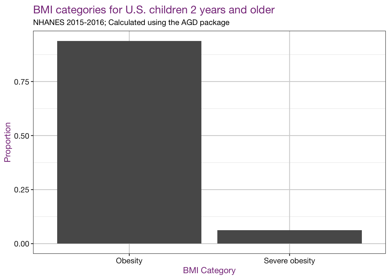
Note: I haven’t taken the complex survey design into account here, so these proportions are not an accurate estimate of the prevalence in the U.S. See this report for those estimates.
growthstandards / hgbd
The growthstandards package, developed by Ryan Hafen, is an offshoot from a larger package, hbgd, and some docs for the growth standards calculations can be found here. It provides calculations for:
- WHO height, weight, head circumference, muacc, subscalpular skinfold, triceps skinfold
- INTERGROWTH fetal head circumference, biparietel diameter, occipito-frontal diameter, abdominal circumference, femur length
- INTERGROWTH newborn (including very preterm) weight, length, and head circumference
The package has some very useful functions for converting units such as:
months2days()for converting age in months to age in days, andlb2kg()for pounds to kilograms.
devtools::install_github("HBGDki/growthstandards")The Center for Disease Control (CDC) and American Academy of Pediatrics (AAP) recommend using the WHO growth standards for children in the United States under 2 years old. To calculate the age- and sex-adjusted BMI z-scores for the children in the NHANES dataset using the WHO reference charts we can do the following:
child_who <- child_df %>%
  filter(agemos < 24) %>%
  mutate(
    bmi = weight_kg/((length_cm/100)^2) ,
    agedays = growthstandards::months2days(agemos),
    # measurements to bmi z-score
    bmiz = growthstandards::who_bmi2zscore(
      agedays = agedays,
      bmi = bmi,
      sex = sex),
    # measurements to percentiles
    bmipct = growthstandards::who_bmi2centile(
      agedays = agedays,
      bmi = bmi,
      sex = sex),
    # find the 95th percentile for age and sex
    p95 = growthstandards::who_centile2bmi(
      agedays = agedays,
      p = 95,
      sex = sex),
    # calculate the percentage of the 95th
    bmipct95 = (bmi/p95)*100,
    # obesity?
    obesity = if_else(bmipct >= 95, 1, 0))
## Registered S3 method overwritten by 'pryr':
## method from
## print.bytes Rcppchild_who %>%
select(bmi, bmiz, bmipct, bmipct95, obesity) %>%
skimr::skim()| Name | Piped data |
| Number of rows | 634 |
| Number of columns | 5 |
| _______________________ | |
| Column type frequency: | |
| numeric | 5 |
| ________________________ | |
| Group variables | None |
Variable type: numeric
| skim_variable | n_missing | complete_rate | mean | sd | p0 | p25 | p50 | p75 | p100 | hist |
|---|---|---|---|---|---|---|---|---|---|---|
| bmi | 4 | 0.99 | 17.24 | 1.67 | 11.63 | 16.17 | 17.17 | 18.34 | 27.77 | ▁▇▃▁▁ |
| bmiz | 4 | 0.99 | 0.57 | 1.03 | -3.62 | -0.05 | 0.57 | 1.23 | 5.56 | ▁▃▇▁▁ |
| bmipct | 4 | 0.99 | 65.78 | 26.93 | 0.01 | 47.82 | 71.54 | 89.13 | 100.00 | ▂▂▃▅▇ |
| bmipct95 | 4 | 0.99 | 91.47 | 8.25 | 64.85 | 86.21 | 90.89 | 96.41 | 142.17 | ▁▇▃▁▁ |
| obesity | 4 | 0.99 | 0.14 | 0.35 | 0.00 | 0.00 | 0.00 | 0.00 | 1.00 | ▇▁▁▁▁ |
Density plots of our new values:
vars <- c("bmi", "bmiz", "bmipct", "bmipct95")
sub <- "Using WHO growth charts from growthstandards package"

density_fun <- function(xvar, df, sub) {
  myplot <- ggplot(df, aes_string(x = xvar)) +
    geom_density() +
    labs(title = paste0("Density plot of ", xvar),
         subtitle = sub) +
    r_ladies_theme()

  plot(myplot)
}

purrr::walk(.x = vars, .f = density_fun, df = child_who, sub = sub)
## Warning: Removed 4 rows containing non-finite values (stat_density).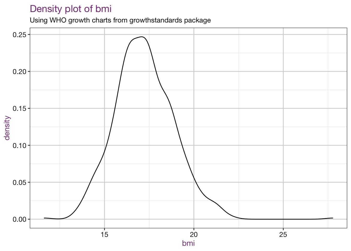
## Warning: Removed 4 rows containing non-finite values (stat_density).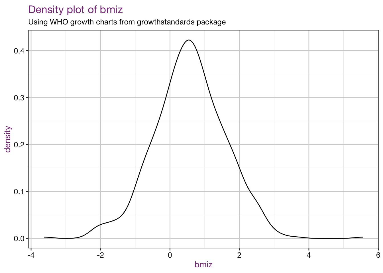
## Warning: Removed 4 rows containing non-finite values (stat_density).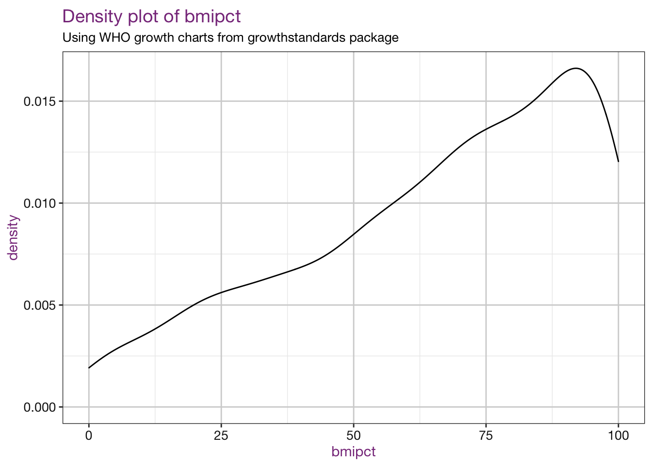
## Warning: Removed 4 rows containing non-finite values (stat_density).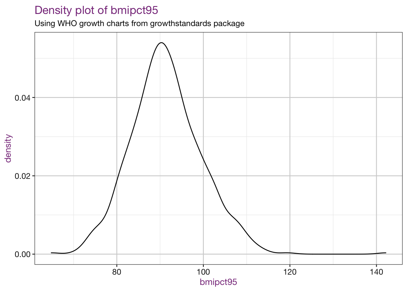
zscorer
The zscorer package is developed by Mark Myatt and Ernest Guevarra.
zscorer refers to the results of the WHO Multicentre Growth Reference Study as standard for calculating the z-scores hence it comes packaged with this reference data.
The WHO Multicentre Growth Reference Study combined longitudinal data for children from birth to 24 months and cross-sectional data for children up to 71 months
install.packages("zscorer")The authors note that:
The function fails messily when secondPart is outside of the range given in the WGS reference (i.e. 45 to 120 cm for height and 0 to 60 months for age). It is up to you to check the ranges of your data.
Because this function is meant for a specific age and height range, I’ll filter the data first.
zscorer_df <- child_df %>%
  filter(agemos < 60) %>%
  filter(height_length_cm < 120,
         height_length_cm > 45) %>%
  select(id, sex_num, height_length_cm, weight_kg, agemos) %>%
  drop_na() %>%
  as.data.frame() # cannot be type tbl_df

library(zscorer)

# height for age z-score
zscorer_df$haz <- getCohortWGS(data = zscorer_df,
                                 sexObserved = "sex_num",
                                 firstPart = "height_length_cm",
                                 secondPart = "agemos",
                                 index = "hfa")
# weight for age z-score
zscorer_df$waz <- getCohortWGS(data = zscorer_df,
                                 sexObserved = "sex_num",
                                 firstPart = "weight_kg",
                                 secondPart = "agemos",
                                 index = "wfa")
# weight fot height z-score
zscorer_df$whz <- getCohortWGS(data = zscorer_df,
                                 sexObserved = "sex_num",
                                 firstPart = "weight_kg",
                                 secondPart = "height_length_cm",
                                 index = "wfh")

zscorer_df %>%
  select(haz, waz, whz) %>%
skimr::skim()| Name | Piped data |
| Number of rows | 1246 |
| Number of columns | 3 |
| _______________________ | |
| Column type frequency: | |
| numeric | 3 |
| ________________________ | |
| Group variables | None |
Variable type: numeric
| skim_variable | n_missing | complete_rate | mean | sd | p0 | p25 | p50 | p75 | p100 | hist |
|---|---|---|---|---|---|---|---|---|---|---|
| haz | 0 | 1 | -0.04 | 1.05 | -3.64 | -0.72 | -0.06 | 0.61 | 3.60 | ▁▃▇▃▁ |
| waz | 0 | 1 | 0.43 | 1.07 | -3.36 | -0.26 | 0.41 | 1.09 | 6.20 | ▁▇▇▁▁ |
| whz | 0 | 1 | 0.62 | 1.05 | -3.48 | -0.03 | 0.55 | 1.24 | 6.46 | ▁▇▇▁▁ |
childsds
The childsds package by Mandy Vogel has child reference data from many other countries (WHO, UK, Germany, Italy, China, and more).
install.packages("chilsds")You can obtain information about the reference data by doing:
childsds::cdc.ref## *** Group of Reference Tables ***
## [1] "CDC containing 8 reference tables"
##
## *** Table of Reference Values ***
## [1] "bmi fitted with: male BCCG, female BCCG"
## sex minage maxage
## male male 2 20.04167
## female female 2 20.04167
##
## *** Table of Reference Values ***
## [1] "height fitted with: male BCCG, female BCCG"
## sex minage maxage
## male male 0 2.958333
## female female 0 2.958333
##
## *** Table of Reference Values ***
## [1] "height2 fitted with: male BCCG, female BCCG"
## sex minage maxage
## male male 2 20
## female female 2 20
##
## *** Table of Reference Values ***
## [1] "weight fitted with: male BCCG, female BCCG"
## sex minage maxage
## male male 0 3
## female female 0 3
##
## *** Table of Reference Values ***
## [1] "hc fitted with: male BCCG, female BCCG"
## sex minage maxage
## male male 0 3
## female female 0 3
##
## *** Table of Reference Values ***
## [1] "wfl fitted with: male BCCG, female BCCG"
## sex minage maxage
## male male 45 103.5
## female female 45 103.5
##
## *** Table of Reference Values ***
## [1] "wfl2 fitted with: male BCCG, female BCCG"
## sex minage maxage
## male male 77 121.5
## female female 77 121.5
##
## *** Table of Reference Values ***
## [1] "weight2_20 fitted with: male BCCG, female BCCG"
## sex minage maxage
## male male 2 20
## female female 2 20
## [1] "Flegal, Katherine M., and T. J. Cole. Construction of LMS Parameters for the Centers for Disease Control and Prevention 2000 Growth Charts. Hational health statitics reports 63."
## [1] "bmi - bmi"
## [1] "height0_3 - height 0 - 3 years old"
## [1] "height2_20 - height 2- 20 years old"
## [1] "weight - - weight 0 - 3 years old"
## [1] "weight2_20 - weight 2- 20 years old"
## [1] "hc - headcircumference"
## [1] "wfl - weight for length"
## [1] "wfl and wfls - age must refer to the length variable; the function gives the sds for a given weight conditional on height"
## [1] "use one of the following keys: bmi - height0_3 - height2_20 - weight - hc - wfl - wfl2 - weight2_20"We can calculate the BMI z-score and percentile given the reference charts using the sds() function:
library(childsds)

childsds_df <- child_df %>%
  filter(agemos >= 24) %>%
  mutate(bmiz = sds(bmi,
                    age = ageyears,
                    sex = sex, male = "Male", female =  "Female",
                    ref = cdc.ref,
                    item = "bmi",
                    type = "SDS"),
         bmipct = round(pnorm(bmiz)*100,2),
         # or use sds function and type = "perc"
         bmipct2 = sds(bmi,
                    age = ageyears,
                    sex = sex, male = "Male", female =  "Female",
                    ref = cdc.ref,
                    item = "bmi",
                    type = "perc")) %>%
  glimpse()
## Rows: 3,426
## Columns: 14
## $ id <dbl> 83738, 83739, 83743, 83745, 83746, 83748, 83749, 837…
## $ agemos <dbl> 141, 54, 217, 185, 52, 41, 210, 196, 182, 194, 235, …
## $ sex_num <dbl> 2, 1, 1, 2, 2, 1, 2, 2, 1, 1, 2, 2, 2, 1, 2, 2, 1, 2…
## $ bmi <dbl> 18.1, 15.7, 26.2, 25.0, 16.1, 16.1, 29.0, 22.2, 24.5…
## $ height_cm <dbl> 143.5, 102.1, 166.1, 169.2, 105.0, 103.6, 161.7, 152…
## $ length_cm <dbl> NA, NA, NA, NA, NA, 104.2, NA, NA, NA, NA, NA, 96.5,…
## $ weight_kg <dbl> 37.2, 16.4, 72.4, 71.7, 17.7, 17.3, 75.9, 51.7, 71.2…
## $ sex_mf <chr> "F", "M", "M", "F", "F", "M", "F", "F", "M", "M", "F…
## $ sex <chr> "Female", "Male", "Male", "Female", "Female", "Male"…
## $ height_length_cm <dbl> 143.5, 102.1, 166.1, 169.2, 105.0, 103.6, 161.7, 152…
## $ ageyears <dbl> 11.750000, 4.500000, 18.083333, 15.416667, 4.333333,…
## $ bmiz <dbl> 0.06918427, 0.16255051, 1.14597646, 1.16637733, 0.63…
## $ bmipct <dbl> 52.76, 56.46, 87.41, 87.83, 73.79, 58.83, 93.97, 68.…
## $ bmipct2 <dbl> 0.5275785, 0.5645638, 0.8740976, 0.8782690, 0.737890…Plot the values:
sub <- "Using CDC growth charts from childsds package"
vars <- c("bmiz", "bmipct")

purrr::walk(.x = vars, .f = density_fun, df = childsds_df, sub = sub)
## Warning: Removed 86 rows containing non-finite values (stat_density).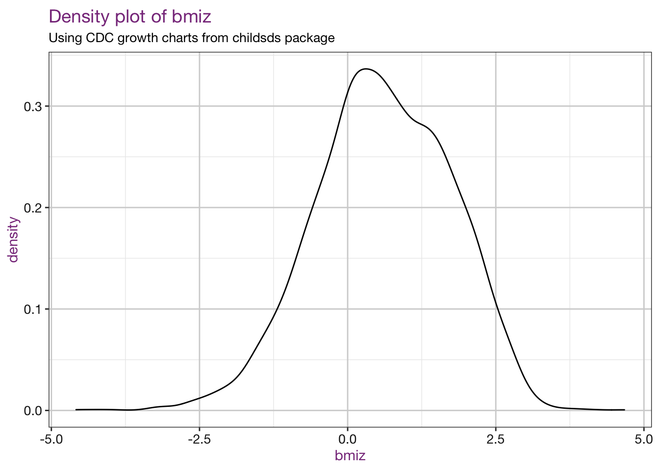
## Warning: Removed 86 rows containing non-finite values (stat_density).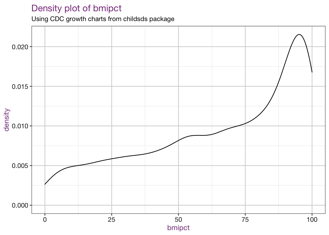
Other work
There is some other publicly available work in this research area:
SITAR: SuperImposition by Translation And Rotation model by Tim Cole and colleagues. The SITAR package provides functions for fitting and plotting growth curve models. More background information can be found here.
Canadian Pediatric Endocrine Group: This group has made available SAS, R, an Stata programs for the WHO growth charts, an R script for waist circumference z-scores (NHANES, cycle III), and an R script for the preterm z-scores (Fenton reference). They have also published many shiny apps!
Please comment if you have found something that I’m missing. I will write a second post with thoughts on what to do next with our unconf project, mchtoolbox.
Thanks Jenny Draper, Jennifer Thompson, Kyle Hamilton, and Charles Gray for being on this team!↩︎